How much should AI enhancement upscale? A bounded design

22 August 2026 · updated 24 August with the tiling & cost measurements · data: decision record, production logs, lab bench

Super-resolution models are quadratic: double the input edge and you quadruple the work — and the wait. Run one naively over whatever people upload and a 40-megapixel scan takes minutes while a phone snap takes seconds. Our enhancement stage instead plans every job so the model's workload is the same bounded size no matter what arrives. This note gives the planning rule, and — new in this revision — the measurements behind its two load-bearing claims: that cost is linear once bounded (~15.6 s per input megapixel on the bench box, r² > 0.999), and that tiled inference is visually seamless only because every tile carries 8 px of context, which removes 87% of the seam energy that zero-padding leaves behind.

2560 pxoutput long-edge targetso the model input is ≤ 640 px

15.6 s/MPmeasured cost, linearr² > 0.999 on the bench box

3.4×seam energy at 0 px paddingboundaries vs surrounding image

87%of excess seam removedby the production 8 px context

Every number in this note was measured on the production pipeline code — same models, same math. Raw per-image records: e6_tiles.json.

1 · The planning rule

The stage targets an output of at most 2560 px on the long edge, using a 4× super-resolution model^[1]. Working backwards, the model never needs an input longer than 2560 ÷ 4 = 640 px, so the planner pre-shrinks whatever arrives to that bound before the model runs — capping the model's input around 0.41 megapixels whether the upload was 1 MP or 40 MP. Formally, for an upload with long edge L:

out = min(4L, 2560), pre = ⌈out / 4⌉, skip if out < 1.3 · L(1)

Three guardrails complete the rule: the output never lands below the original resolution (enhancement must never cost you pixels), inputs already near or above the target skip the pass entirely — the 1.3× minimum-gain clause, because below that the resample-and-model round trip blurs about as much as it sharpens — and faces are restored after the pass, so face crops enter the face model at the improved resolution.

8211024

Upload0.84 MP

513640

Model input (pre-shrunk)0.33 MP

20522560

Output (×4)5.25 MP

Figure 1. The bounded plan for the benchmark scan: the model sees a 0.33 MP input regardless of upload size; its 4× output lands exactly on the 2560 px target.

2 · Why a bound at all: cost is linear — after you make it so

The claim that motivates the whole design is measurable, so we measured it: the production upscale path (192 px tiles, 8 px padding, ONNX Runtime CPU^[3]) run over inputs from 0.04 to 0.39 megapixels on 2-vCPU container-class hardware:

Figure 2. Wall-clock vs input megapixels through the production tile path. The fit is linear at ≈15.6 s per input megapixel (r² > 0.999). Linear in input pixels is still quadratic in edge length — which is exactly why the planner bounds the edge before the model runs: the bound turns “could take minutes” into “always a few seconds of model time.”

A second engineering fact falls out of the same sweep: total runtime is essentially independent of tile size (96 → 384 px all land within 8% of each other) — the work is per-pixel, and the padding overhead at 8 px is noise. Tile size is therefore chosen for memory, not speed: 192 px keeps the peak tensor small enough for the browser fallback engine's WASM heap.

3 · The seam tax, and why 8 px of context pays it

Tiling has a failure mode the papers rarely dwell on: convolutions have receptive fields, so a tile cut with no surrounding context is wrong along its border, and the reassembled mosaic shows a grid. We measure it with a seam index — mean luma gradient across tile-boundary pixel columns divided by the mean gradient elsewhere; 1.0 means boundaries are statistically invisible:

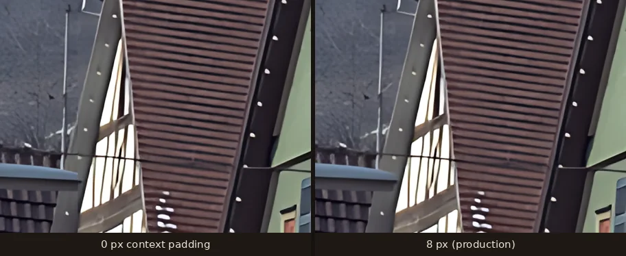
Figure 3. Seam index vs context padding, 192 px tiles on a texture-dense Kodak frame. Zero padding leaves tile boundaries 3.4× busier than the surrounding image — visible stripes on the output grid. Eight pixels — the production setting — removes 87% of the excess; sixteen buys only three points more for double the padding compute.

Two upscaled crops of window shutters; the unpadded version shows visible vertical seam lines that the padded version does not — Figure 4. The same reconstruction with 0 px (left) and 8 px (right) of tile context. The left panel's repeating discontinuities sit exactly on the output's tile grid — each tile judged the edge of its world differently.

The shape of that curve is the design argument in miniature: the first two pixels of context buy half the improvement, eight buys diminishing returns, and past eight you are paying quadratic-ish padding overhead for seam energy no viewer can find. (Whether the enhanced pixels themselves beat classical interpolation is a separate question with a measured answer — see the 28-image benchmark, where the model gives up 1.07 dB of PSNR to Lanczos-3 and restores 3.1× the edge energy^[2].)

4 · Measured timings, end to end

Benchmark: an 821×1024 black-and-white scan restored to 2052×2560, colourised, one face, on a warm instance.

Colourise1.5 s

Enhance (bounded)2.9 s

Face restore1.8 s

Figure 5. Per-stage wall-clock on the warm benchmark run, 6.4 s total. The bounded enhancement pass is not the dominant stage.

End to end in production on the same photo: 68 s on a cold start (model weights loading) and 32 s warm. For scale: the previous pipeline, which upscaled nothing and only touched faces, ran 23–34 s warm — the bounded whole-image pass adds almost nothing to the wall clock, because its input is small by construction. And when the same job runs inside the browser (the automatic fallback), a 1000×1223 scan took 340.8 s on an Apple-silicon desktop with WebGPU — same bounded plan, roughly 10× the wall clock. The bound is what keeps even that worst case usable rather than unbounded.

5 · What was rejected

Diffusion-based super-resolution (far too slow for an interactive tool on our stack), larger per-face restoration models as the default (per-face time balloons on group photos), and sending photos to external GPU inference APIs — photos would leave our infrastructure, which the privacy promise rules out. The bounded plan keeps quality gains where a viewer actually perceives them — a screen-sized image — instead of paying quadratically for pixels nobody can see.

6 · Limitations

The 2560 px target is a product decision, not an optimum: prints benefit from more resolution, and a future paid tier could raise the bound. The timings above are the common case — photos dense with faces spend proportionally more in the face stage, which the enhancement bound does not cover. And the seam index is a statistical instrument: it certifies boundaries are quiet on average, not that no adversarial texture could ever reveal one.

References

Wang, X., Xie, L., Dong, C., & Shan, Y. (2021). Real-ESRGAN: Training Real-World Blind Super-Resolution with Pure Synthetic Data. ICCV Workshops. arXiv:2107.10833. arxiv.org
Kodak Lossless True Color Image Suite — 24 uncompressed 768×512 PhotoCD reference images, the classic image-quality test set. r0k.us
ONNX Runtime — the inference engine both our server (CPU) and in-browser (WebGPU/WASM) engines run on. onnxruntime.ai