AI upscaling vs bicubic: a 28-image benchmark
Every photo tool now promises to “enhance.” Ours runs Real-ESRGAN[1], so we owed an uncomfortable question an answer: when you measure the way the image-processing literature measures, does the AI actually beat plain bicubic interpolation? The result is the most interesting kind of answer (no, and also emphatically yes), and the split between those two answers has a name in the literature: the perception–distortion tradeoff[3]. This note shows the full benchmark, including the case where the AI loses badly (film grain), and why we ship the model that loses the classical benchmark anyway.
Every number in this note was measured on the production pipeline code: same models, same math. Raw per-image records: e1_sr.json.
1 · Method
The corpus is the 24-image Kodak Lossless True Color Suite[4] (the 768×512 reference set the compression and super-resolution literature has leaned on for three decades), plus four 768×512 crops from high-resolution scans of historical photographs, including Dorothea Lange's 1936 Migrant Mother[5], because this site exists for old photos and old photos have film grain. That distinction decides Section 3.
We score three things. Fidelity, as peak signal-to-noise ratio over RGB:
structural similarity (SSIM[2], luma, the standard 11×11 Gaussian window, σ = 1.5, K₁ = 0.01, K₂ = 0.03):
and sharpness as the Tenengrad measure (mean squared Sobel gradient magnitude), reported as a restoration ratio, Tenengrad(output) ÷ Tenengrad(ground truth). A ratio of 1.0 would mean the reconstruction carries as much edge energy as the original photograph.
2 · Results: the tradeoff, live
On the metric everyone reports, the classical ladder behaves exactly as sampling theory predicts (each better kernel buys a fraction of a decibel), and Real-ESRGAN comes last but one:
| Method | PSNR (dB) | σ | SSIM | Tenengrad ratio | ms / image* |
|---|---|---|---|---|---|
| Nearest neighbour | 25.42 | ±3.42 | 0.673 | 0.382 | 8 |
| Bilinear | 25.88 | ±3.62 | 0.687 | 0.152 | 236 |
| Bicubic (Catmull-Rom) | 26.29 | ±3.68 | 0.705 | 0.196 | 343 |
| Lanczos-3 | 26.45 | ±3.71 | 0.711 | 0.216 | 876 |
| Real-ESRGAN ×4 (ours) | 25.38 | ±3.16 | 0.711 | 0.676 | 462 |
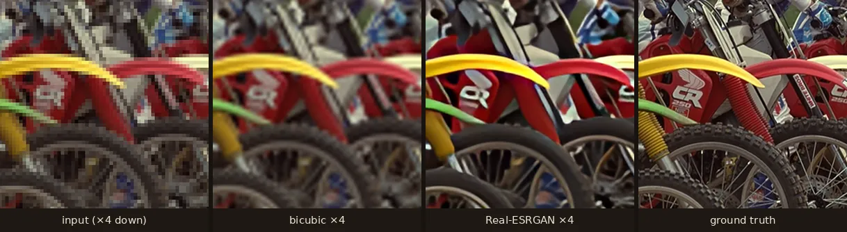
*192×128 input, 2-vCPU container-class hardware; ratios transfer, milliseconds don't. If PSNR were the whole story we would ship Lanczos-3 and delete 4.9 MB of neural network. But plot each method on the fidelity axis against the sharpness axis and the field splits into two species:
SSIM (designed to track perceived structure rather than raw error[2]) splits the difference and sides, narrowly, with the model: best mean of the field overall, and a clearer 0.704 vs 0.694 on the Kodak subset where fine texture dominates. Why can't interpolation compete on sharpness? Because every classical kernel is a linear, shift-invariant operator: it can only redistribute the frequencies that survived downsampling, never create the ones that didn't. The Nyquist limit is not a suggestion. A GAN prior sidesteps the limit by changing the question: from “what signal produced these samples?” (unanswerable) to “of all the natural images that would downsample to this, which is most plausible?”[1] That is also exactly where its risk lives: plausible is not true.
3 · The film-grain problem, quantified
Averages hide the most useful finding. Split the corpus and the per-image PSNR deltas (Real-ESRGAN − Lanczos-3) are sharply bimodal: on clean modern frames the model is within a decibel (it beats Lanczos outright on one, +0.15 dB); on the four historical film scans it loses catastrophically: the subset means are 28.75 vs 32.12 dB:
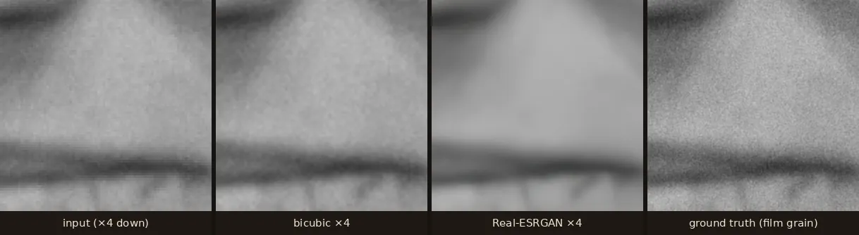
Under a loupe the numbers become obvious: the ground-truth scan is a wall of honest grain, and the model returns porcelain. On Migrant Mother it drops 1.71 dB and 0.064 SSIM, and some viewers will still prefer the clean output. Metrics are not taste; they are a contract about which taste you are optimizing. This measurement is why the enhancement stage skips photos already near its resolution target (a high-resolution archival scan keeps its native pixels and its grain), and why our face rendering blends the photograph's own grain back over restored faces instead of shipping the model's porcelain.
4 · Limitations
- No learned perceptual metric. LPIPS or DISTS would sharpen the perception axis; Tenengrad is an honest but simpler proxy. The raw records are published so anyone can re-score.
- One degradation. Bicubic ×4 is the standard protocol and the kindest case; real scans add blur kernels, JPEG, and noise (the face note uses the full corruption stack).
- N = 28: plenty for these effect sizes (the ordering is stable under leave-one-out), small for subgroup claims beyond the grain split.
5 · Conclusion
Measured as signal reconstruction, AI super-resolution is a worse interpolator than Lanczos-3: 1.07 dB worse here, exactly as the perception–distortion tradeoff predicts[3]. Measured as photograph reconstruction (structure, edge energy, and your eyes) it is not close, in the other direction. The practical reading for your shoebox: for photos that will be viewed by people, the model is the right default; for archival masters where every grain particle is evidence, keep the raw scan too. The restore tool is built around exactly that split.
References
- Wang, X., Xie, L., Dong, C., & Shan, Y. (2021). Real-ESRGAN: Training Real-World Blind Super-Resolution with Pure Synthetic Data. ICCV Workshops. arXiv:2107.10833. arxiv.org
- Wang, Z., Bovik, A. C., Sheikh, H. R., & Simoncelli, E. P. (2004). Image Quality Assessment: From Error Visibility to Structural Similarity. IEEE Transactions on Image Processing, 13(4), 600–612. doi.org
- Blau, Y., & Michaeli, T. (2018). The Perception-Distortion Tradeoff. CVPR. arXiv:1711.06077. arxiv.org
- Kodak Lossless True Color Image Suite: 24 uncompressed 768×512 PhotoCD reference images, the classic image-quality test set. r0k.us
- Lange, D. (1936). “Migrant Mother” (Destitute pea pickers in California), Farm Security Administration. Public domain, via Wikimedia Commons. commons.wikimedia.org
- ONNX Runtime: the inference engine both our server (CPU) and in-browser (WebGPU/WASM) engines run on. onnxruntime.ai